Hybrid linear-nonlinear optimization approach to the approximation of multi-pole Debye dielectric function

In electromagnetism, a dielectric medium is a type of insulator, which can be polarized by applying an electric field. The dielectric polarisation is caused by the slight movement of the electric charges inside (positive one in the direction of the external field, negative - opposite). This creates an internal electric field, and in some cases can also reorient the molecules of the material. To measure the electric polarizability of the material, the variable called permittivity is used (denoted by the Greek letter ε (epsilon)). A material with high permittivity polarizes more in response to an applied electric field than a material with low permittivity, thereby storing more energy in the material. The study of dielectric properties concerns the storage and dissipation of electrical and magnetic energy in materials, and is important to explain various physical phenomena.
Some materials show dielectric dispersion. It means that the permittivity of dielectric material depends on the frequency of an applied electric field. This frequency dependence reflects the fact that a material's polarization does not change instantaneously when an electric field is applied. The response of the material always arises after the applied field, and in case of an oscillating electric field gives a rise of a characteristic dielectric relaxation process [1]..

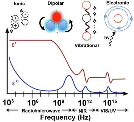
A dielectric permittivity spectrum over a wide range of frequencies. ε′ and ε″ denote the real and the imaginary part of the permittivity, respectively. Various processes that influence the response of a material are labeled on the image. Image by [1].

Variants of the relaxation functions

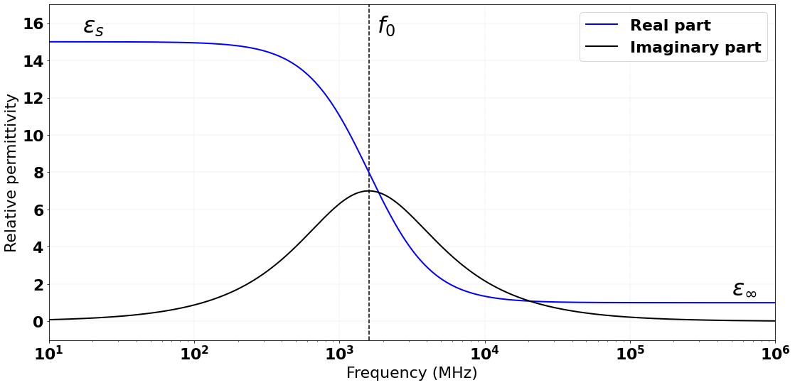
Debye equation models relaxation processes in alternating electric fields of angular frequency ω, describing the dielectric relaxation response of an ideal, noninteracting population of electric dipoles. Taking as basic principle that the polarization decays exponentially, the complex permittivity is given by Debye's function as [2]

Here, the real part ε′(ω) is the permittivity and the imaginary part ε″(ω) is the loss factor, and i = √–1. εs is the static permittivity, ε∞ is the infinite-frequency permittivity, and τo is the relaxation time, which is the characteristic time for the relaxation process.

A dielectric permittivity spectrum over a wide range of frequencies. ε′ and ε″ denote the real and the imaginary part of the permittivity, respectively. Various processes that influence the response of a material are labeled on the image. Image by [1].

However, the single-pole Debye equation is a poor model of dielectric behavior for most materials over wide frequency ranges. To overcome this, empirically derived Havriliak–Negami relaxation was proposed as modification of the single-pole Debye relaxation model. The equation additionally has two exponential parameters, and is expressed as [3]

where α and β are positive real constants (0 ≥ α, β ≤ 1). From this model, the Cole-Cole equation [4] setting β=1, and Cole-Davidson equation [5] forα= 1can be derived. TheDebye equation is obtained with α=1and β=1. The Havriliak-Negami function was first used to describe the dielectric properties of polymers [3], whereas the Cole-Cole equation is mainly used to model biological tissues [6] and liquids [7].
On the other hand, Jonscher function in the constant Q-factor approach (or quality Q-factor) [8] is mainly used to describe the dielectric properties of concrete [9] and soils [10]. Other types of relaxation functions estimate the bulk permittivity of heterogeneous materials.In the task, the Complex Refractive Index Model (CRIM) [11] illustrates the dielectric properties of the mixture with respect to the dielectric properties and the volumetric fractions of its components.
Havriliak-Negami, Jonscher function as well as steady Q-factor, CRIM, and experimentally obtained data cannot be directly implemented to the FDTD algorithm. An approach used by many researchers is approximation of the complex permittivity using multi-pole Debye expansion with multiple relaxation times and a dimensionless weights in form [12]

being εn and τ0,n= 1,2,...,N the change in the permittivity (weights) and relaxation times of the Debye dispersion, respectively. Parameter indicates number of Debye poles (the total number of Debye expansion components). The multi-pole Debye model is widely used since it can easily be expressed in both time and frequency domains.

Finding relaxation times and a dimensionless weights

The objective of the multi-pole Debye fitting process is to minimize the objective function, which is the difference between the chosen relaxation model (here we have Havriliak-Negami, Jonsher, CRIM or experimental data) and approximate form of Debye expansion. The function in the task is clearly defined, including twice as many variables as the number of Debye poles, since we want to calculate both relaxation times, and dimensionless weights.
Because of the causal nature of dispersive materials, the real and imaginary parts of the permittivity are related to each other via the Kramers-Kronig relations.This suggests that the real and imaginary parts of the permittivity supposed to be closely approximated by a sum of Debye function for the same parameters. Then, the optimization procedure could be done only for the real-valued expansion of the imaginary part. In literature some single nonlinear optimization procedures are used to find all of the unknown parameters (namely the weights and relaxation times). However, because the expansion is a linear combination of Debye functions, a more efficient approach is to find the weights using a linear least squares (LS) method and the relaxation frequencies using a nonlinear method (here the Particle Swarm Optimization (PSO) technique is used as a default).

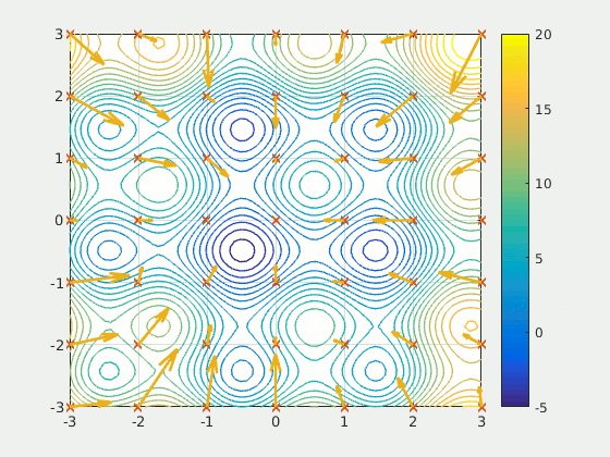
Finding the global minimum of the function using the PSO algorithm. Image by Wikimedia Commons.

The technique employed in the gprMax subpackage DebeFit is a modification of the hybrid linear-nonlinear optimisation method proposed by Kelley et al. [13]. The adjustments allowed to overcome some instability issues and thus making the process more robust and faster. In particular, in the case of negative weights the sign is inverted in order to introduce a large penalty in the optimisation process (thus indirectly constraining the weights to be always positive). This made dumbing factors unnecessary and consequently they were removed from the algorithm. Furthermore the difference between approximated and calculated real part of dielectric permittivity was added to the cost action to avoid possible instabilities.

Code structure

The gprMax subpackage DebeFit contains two main scripts:

• Debye_fit.py with definition of all Relaxation functions classes,
• optimization.py with definition of three chosen global optimization methods.
  The Class Relaxation is designed for modelling different relaxation functions, like Havriliak-Negami (Class HavriliakNegami), Jonscher (Class Jonscher), Complex Refractive Index Mixing (Class CRIM) models, and arbitrary dielectric data derived experimentally or calculated using some other function (Class Rawdata). The constructor for chosen object type constructs a proper relaxation object and defines all its parameters, along with frequency point grid. The Class Optimizer supports global optimization algorithms (particle swarm, duall annealing, evolutionary algorithms) for finding an optimal set of relaxation times that minimise the error between the actual and the approximated electric permittivity and calculate optimised weights for the given relaxation times. Code written here is mainly based on external libraries, like scipy and pyswarm. The optimizer object is created inside the relaxation module. The user has the possibility to choose one from three optimization algorithms and its properties in the form of a python dictionary.
  The fitting procedure is launched after relaxation object initialization, by using the run method. Algorithm implemented inside the function consists of the following steps:

1. Check the validity of the inputs using the check_inputs method.
2. Print information about chosen approximation settings using the print_info method.
3. Calculate both real and imaginary parts using the calculation method, and then set self.rl and self.im properties.
4. Call the main optimization module using the optimize method and calculate errors based on the error method. [OPTIONAL] If number of debye poles is set to -1 optimization procedure is repeated until percentage error goes smaller than 5% or 20 Debye poles is reached.
5. Print the results in gprMax format style using the print_output method.
6. [OPTIONAL] Save results in gprMax style using the save_result method.
7. [OPTIONAL] Plot the actual and the approximate dielectric properties using plot_result method.

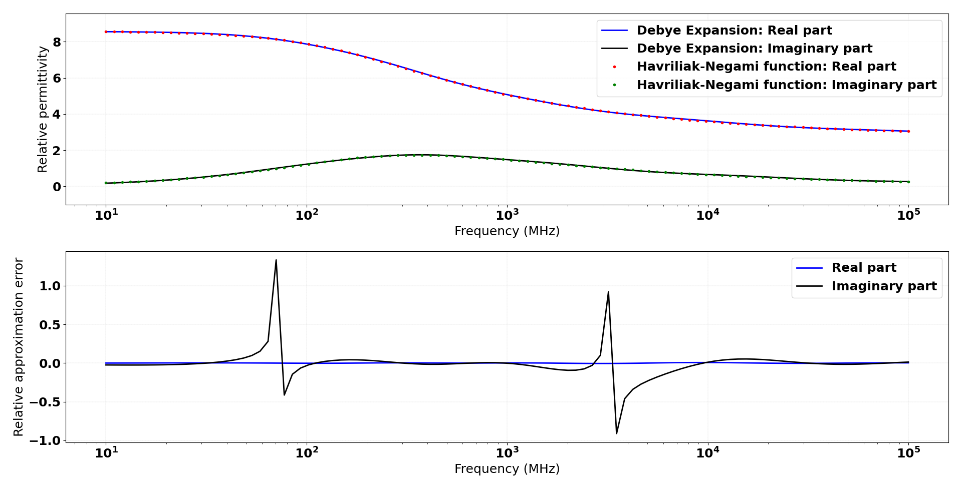
At the end user can plot the actual and the approximate electric permittivity along with the error depending on the frequency.

Summing up

Working for gprMax is a great learning experience. gprMax is a powerful tool to build large and complex simulations of GPR. Its usefulness is confirmed by its widespread use in many areas.
This work describes the addition of new advance modelling features such as the possibility to fit arbitrary dielectric data derived experimentally or calculated using some relaxation function. The hybrid linear-nonlinear optimisation approach employed here provides an effective, and accurate optimisation procedure to fit a multi-pole Debye expansion to dielectric data.

Literature

[1] Application Note 1217-1, Basics of measuring the dielectric properties of materials, Hewlett Packard literature number 5091-3300E, 1992.

[2] P. Debye, Polar Molecules, Dover Publications, New York, 1929.

[3] S. Havriliak, and S. Negami, A complex plane representation of dielec-tric and mechanical relaxation processes in some polymers, Polymer,vol. 8, pp. 161–210, 1967.

[4] K. S. Cole, and R. H. Cole, Dispersion and absorption in dielectrics,alternating current characteristic, Journal of Chemical Physics, vol. 9,pp. 341–351, 1941.

[5] M. F. Manning and M. E. Bell, Electrical conduction and related phenomena in solid dielectrics, Rev. Mod. Phys., vol. 12, pp. 215–257,1940.

[6] D. Ireland, A. Abbosh, Modeling Human Head at Microwave Frequen-cies Using Optimized Debye Models and FDTD Method, IEEE Trans.Antennas and Propagation, vol. 61, no. 4, pp. 2352–2355, 2013.

[7] J. Barthel, R. Buchner, and M. Munsterer, “Electrolyte Data Col-lection, Part 2: Dielectric Properties of Water and Aqueous Elec-trolyte Solutions,” ser. Chemistry Data Series. Frankfurt am Mein, Germany:DECHEMA, vol. XII, 1995.

[8] M. Bano, Modelling of GPR waves for lossy media obeying a cou-plex power law of frequency for dielectric permittivity, GeophysicalProspecting, vol. 41, pp 11–26, 2004.

[9] T. Bourdi, J. Rhazi, F. Boone, and G. Ballivy, Application of Jonschermodel for the characterization of the dielectric permittivity of concrete, Journal of Physics D: Applied Physics, vol. 41, pp. 205410, October 2008.

[10] E. Kjartansson, Constant Q-wave propagation and attenuation, Journal of Geophysical Research, vol. 84, pp. 4737–4748, 1979.

[11] J. R. Birchak, C.G. Gardner, J.E. Hipp, J.M Victor, High dielectric constant microwave probes for sensing soil moisture, Proc. IEEE, vol.62, pp. 93–98, 1974.

[12] C. A. Balanis, Advanced Engineering Electromagnetics, New York : Wiley, Sec. 2.8.1, 1989.

[13] D. F. Kelley, T. J. Destan and R. J. Luebbers, Debye Function Expansions of Complex Permittivity Using a Hybrid Particle Swarm-Least Squares Optimization Approach, IEEE Transactions on Antennas and Propagation, vol. 55, no. 7, pp. 1999–2005, July 2007.